Basic Building Blocks of K-Means Clustering Algorithms

1. Introduction

In the vast sea of data that surrounds us, the ability to uncover patterns and groupings is not just valuable; it’s a necessity for making informed decisions. This is where the K-means algorithm, a stalwart of machine learning, shines by offering a simple yet powerful method for data clustering. Whether you’re a data scientist or just data-curious, understanding K-means can provide new insights from the data you encounter daily.

What is K-means?

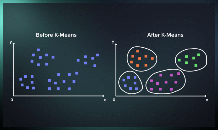
At its core, the K-means algorithm is a method to automatically partition a dataset into distinct groups, or clusters, based on similarity. It’s a building block of unsupervised learning, tasked with finding structure in unlabeled data. By grouping data points into clusters where members are more similar to each other than to those in other clusters, K-means provides a clear view of your data’s natural divisions.

Definition of K-means Clustering

Clustering stands as a pivotal method in exploratory data analysis, offering insights into the underlying structure of datasets. Essentially, it involves grouping data points into subgroups, or clusters, based on their similarity. The aim is to ensure that members within a cluster share a high degree of resemblance, while those in different clusters exhibit distinct differences. This process hinges on selecting an appropriate similarity measure, like Euclidean or correlation-based distance, which can vary depending on the specific application.

Importance and Applications of K-means Clustering

The utility of clustering extends across various domains. For instance, in market segmentation, it helps identify customer groups with similar behaviors or attributes. In the group of image processing, it aids in segmenting and compressing images by grouping similar regions. Additionally, it’s instrumental in organising documents by topics, enhancing our understanding and management of large datasets.

2. Theoretical Background

The theoretical foundation of clustering lies in partitioning data into subsets. This partitioning is based on the concept of similarity, which is quantified through various metrics. The main goal is to maximise the similarity of objects within a cluster and minimise the similarity of objects between different clusters. The effectiveness of a clustering algorithm can largely depend on the context of the application, including the nature of the data and the specific requirements of the task at hand.

Principles of Clustering

Clustering relies on a few key ideas:

1. Similarity Measurement: A most important step in clustering is defining a similarity metric, which quantifies how alike two data points are. This metric directly influences the formation of clusters.
2. Feature Selection: Choosing the right set of features is essential, as it affects the similarity measurements. Irrelevant or noisy features can lead to poor clustering performance.
3. Algorithm Selection: Different algorithms are suited to different types of data and clustering objectives. Choosing the right algorithm is key to obtaining meaningful clusters.
4. Evaluation: Assessing the quality of the clusters formed is vital for verifying the effectiveness of the clustering process. This often involves metrics that measure the cohesion of clusters and the separation between them.

Similarity Measures

The choice of similarity measure is critical in clustering. In K-means, the similarity between data points is typically assessed using Euclidean distance, measuring the straight-line distance between points in space. However, other measures can be used depending on the nature of the data:

• Euclidean Distance: Ideal for continuous data, where the geometric distance is meaningful.
• Cosine Similarity: Used for text data or high-dimensional data, focusing on the angle between vectors rather than their magnitude.
• Manhattan Distance: Useful for ordinal or discretely-valued data, based on the sum of absolute differences.

Each similarity measure has its context where it performs best, and the choice of measure can significantly impact the results of clustering.

3. K-means Algorithm

Algorithm ensures that each piece of data is assigned to a single cluster, aiming to enhance the uniformity within clusters while maintaining clear distinctions between them. The essence of this algorithm is to optimise the allocation of data points to clusters in such a way that the cumulative squared distance from each point to the center of its cluster (the centroid) is minimised. A successful outcome is marked by high similarity among members of the same cluster and notable differences between separate clusters.

Executing the K-means Algorithm involves a series of steps:

1. Selection of Cluster Count: Deciding on the number of clusters, denoted as K.
2. Centroid Initialisation: The dataset is first mixed and then K data points are chosen at random as the initial centroids, ensuring no repetitions.
3. Iterative Optimisation: The algorithm repeatedly adjusts the assignments and centroids until the centroids stabilise, showing no further changes in their positions.
4. Distance Calculation: It computes the total squared distance between the data points and each centroid.
5. Cluster Assignment: Data points are affiliated with the nearest centroid, signifying their cluster membership.
6. Centroid Recalculation: The algorithm recalculates the position of each centroid by averaging the coordinates of all the points in the cluster, refining the cluster’s coherence.

Expectation-Maximisation

The K-means algorithm adopts the Expectation-Maximisation (E-M) strategy to partition data into clusters. This process alternates between two key steps: the expectation (E) step, which involves assigning data points to the nearest cluster, and the maximization (M) step, which computes the centroids of these clusters. Let’s get into the mathematical framework underpinning this approach.

Objective Function

The objective of K-means is encapsulated in the function J, defined as: In this equation, Wik serves as an indicator variable that equals 1 if the data point Xi is allocated to cluster k, and 0 otherwise. The symbol μk denotes the centroid of the cluster that data point Xi is associated with.

E-step (Expectation Step)

During the E-step, the algorithm updates Wik by assigning each data point Xi to the cluster with centroid μk that minimises the squared Euclidean distance. ∥xi−μk∥^2.

M-step (Maximisation Step)

In the M-step, K-means recalculates the centroids μk for each cluster based on the new assignments from the E-step. The updated centroid is computed as the mean of all points assigned to the cluster:

This step ensures that the centroids accurately reflect the current makeup of their clusters, improving the algorithm’s partitioning with each iteration.

Standardisation of Data

• Why It’s Necessary: Clustering algorithms, including K-means, utilize distance metrics to determine the similarity between data points. When features in a dataset are on different scales (for example, age in years and income in thousands of dollars), it can distort the distance measurements, heavily biasing the algorithm towards the larger-scale features. This can lead to misleading clustering results.
• Recommended Approach: To counteract this issue, it’s recommended to standardize the data before clustering. Standardization involves adjusting the data such that each feature has a mean of zero and a standard deviation of one. This process ensures that all features contribute equally to the distance calculations, allowing for a fair comparison of similarities across different dimensions.

Initialisation Sensitivity

• The Challenge: The K-means algorithm begins with a random initialisation of centroids (the starting points of clusters). Due to its iterative nature and reliance on these initial centroids, K-means can converge to different local optima depending on the starting conditions. This means that different initialisations can lead to different clustering outcomes, some of which may be suboptimal.
• Mitigation Strategies: To address this variability and increase the chances of finding a more globally optimal solution, it’s advisable to run the K-means algorithm multiple times with different random initializations of centroids. After these runs, the outcome that yields the lowest sum of squared distances (a measure of how compact the clusters are) should be selected. This approach helps mitigate the impact of unfortunate initial placements and leverages the algorithm’s stochastic nature to explore a broader range of potential solutions.

Convergence and Within-Cluster Variation

• Observing Convergence: The convergence of the K-means algorithm is typically determined when there’s no significant change in the assignment of examples to clusters, indicating stability in the solution. This stability is often measured as minimal or no change in within-cluster variation, which implies that further iterations do not meaningfully alter the structure of the clusters.
• Practical Implication: While the convergence criterion is a useful indicator of algorithm stability, it’s essential to remember that convergence to a stable solution does not necessarily mean that the solution is the best or most meaningful clustering of the data. It merely indicates that the algorithm has found a locally optimal arrangement of data points into clusters based on the initial conditions and distance metrics used.

Implementing K-means in Python

Below is a Python implementation of the K-means clustering algorithm, including data generation and visualization of the resulting clusters.

import numpy as np
import matplotlib.pyplot as plt
import pandas as pd        

#creating KMeans
class K_Means:
    def __init__(self, k=3, tolerance=0.0001, max_iterations=500):
        # the number of clusters to form as well as the number of centroids to generate.
        self.k = k
        # the percentage change in the centroids before considering the algorithm has converged.
        self.tolerance = tolerance
        # the maximum number of times the algorithm will attempt to converge before stopping.
        self.max_iterations = max_iterations

    # method to fit model inside dataset
    def fit(self, data):
        # initialise Centroids Randomly
        # empty dictonary to store centroids
        self.centroids = {}
        # for loop to iterate inside k
        for i in range(self.k):
            self.centroids[i] = data[i]
        # loop through max iterations times
        for i in range(self.max_iterations):
            # create empty classes for each centroid
            self.classes = {i: [] for i in range(self.k)}
            # assigning data points to nearest centroid
            for features in data:
                # euclidean distance between the current data point and each centroid
                distances = [np.linalg.norm(features - self.centroids[centroid]) for centroid in self.centroids]
                classification = distances.index(min(distances))
                self.classes[classification].append(features)
            # previous centroids
            previous = dict(self.centroids)
            # update centroids as mean of assigned data points
            for classification in self.classes:
                self.centroids[classification] = np.mean(self.classes[classification], axis=0)
            # convergence
            isOptimal = True
            for centroid in self.centroids:
                original_centroid = previous[centroid]
                curr = self.centroids[centroid]
                if np.sum((curr - original_centroid) / original_centroid * 100.0) > self.tolerance:
                    isOptimal = False
            # break loop if converged
            if isOptimal:
                break
    # method to predict
    def prediction(self, data):
        # euclidean distance
        distances = [np.linalg.norm(data - self.centroids[centroid]) for centroid in self.centroids]
        classification = distances.index(min(distances))
        return classification        

# generating dataset for testing
np.random.seed(42)
# creating data from random numbers
data = np.random.randn(500, 2)
# standard scale
data = (data - data.mean())/data.std()
print(data[:10])        

# K_Means for the clustering
km = K_Means(3)
# fitting model
km.fit(data)
# checking centroids
km.centroids        

4. Choosing the Number of Clusters

The Elbow Method

The Elbow Method is a heuristic used to determine the optimal number of clusters by plotting the within-cluster sum of squares (WCSS) against the number of clusters. The WCSS decreases as the number of clusters increases because the clusters are smaller and the data points are closer to the centroids. The goal is to identify the point where the decrease in WCSS begins to slow down, which is indicative of diminishing returns by increasing K. This point resembles an “elbow” in the plot, hence the name. The Elbow Method is intuitive and easy to implement but can sometimes be ambiguous if the “elbow” is not very clear.

The Silhouette Method

The Silhouette Method provides a more nuanced approach by measuring how similar an object is to its own cluster compared to other clusters. The silhouette score ranges from -1 to 1, where a high value indicates that the object is well matched to its own cluster and poorly matched to neighboring clusters. For each K, you calculate the average silhouette score of all objects. The optimal number of clusters corresponds to the K with the highest average silhouette score. This method not only helps in determining the number of clusters but also provides insight into the separation distance between the resulting clusters, offering a more detailed perspective on cluster cohesion and separation.

Other Methods for Determining the Optimal K

Besides the Elbow and Silhouette Methods, several other techniques can help in deciding the optimal number of clusters:

• Gap Statistic: Compares the total within intra-cluster variation for different values of K with their expected values under null reference distribution of the data. The gap statistic measures the gap between the logarithm of within-cluster dispersion and its expectation under a reference null distribution. The optimal K is the one that maximizes this gap.
• Davies-Bouldin Index: Aims to identify the number of clusters that minimize the average ‘similarity’ between clusters, where similarity is a measure that compares the distance between clusters with the size of the clusters themselves. A lower Davies-Bouldin Index indicates a better partitioning.
• Akaike Information Criterion (AIC) or Bayesian Information Criterion (BIC): Used in mixture-model based clustering, these criteria evaluate the model fit of the clustering solution while penalizing for the number of parameters to avoid overfitting. The optimal K is the one that minimizes the AIC or BIC.

Visualizing Clusters in Python

The following code demonstrates how to visualize the clusters and centroids generated by the K-means algorithm, along with the Elbow Method to determine the optimal number of clusters.

def within_cluster_sum_of_squares(data, k):
    kmeans = K_Means(k)
    kmeans.fit(data)
    wcss = sum([np.sum([np.linalg.norm(x - kmeans.centroids[ci])**2 for x in kmeans.classes[ci]]) for ci in kmeans.classes])
    return wcss        

def clustering(km, x1, x2):
    plt.figure(figsize=(10, 6))
    # total colors for plotting clusters
    colors = ["black", "green", "cyan", "orange", "blue", "magenta", "yellow", "white", "purple", "brown", "pink"]
    # iterate over each cluster
    for classification in km.classes:
        color = colors[classification]
        for features in km.classes[classification]:
            # plotting each data point in the cluster
            plt.scatter(features[0], features[1], color=color, s=30, alpha=0.5)
    # initialise centroid label counter
    centroid_label = 1
    # iterate over each centroid and plot them with number labels
    for centroid in km.centroids:
        # plotting centroid of cluster
        plt.scatter(km.centroids[centroid][0], km.centroids[centroid][1], s=300, marker="X", color='red')
        # text label at centroid center
        plt.text(km.centroids[centroid][0], km.centroids[centroid][1], str(centroid_label), ha='center', va='center', color='white', fontsize=12, fontweight='bold')
        # increment centroid label counter
        centroid_label += 1
    plt.grid(True, ls='--', alpha=0.2, color='grey')
    plt.title("K-Means Clustering")
    plt.xlabel(f"{x1}")
    plt.ylabel(f"{x2}")
    plt.show()

# calling function for plot
clustering(km, "feature1", "feature2")

def elbow(data):
    # K values range from 1 to 10
    k_values = range(1, 10)
    # formula for within-cluster sum of squares
    wcss_scores = [within_cluster_sum_of_squares(data, k) for k in k_values]
    plt.figure(figsize=(8, 4))
    plt.plot(k_values, wcss_scores, '-o', color='red')
    plt.title('Elbow Method For Optimal k')
    plt.xlabel('Number of clusters k')
    plt.ylabel('Within-Cluster Sum of Squares')
    plt.xticks(k_values)
    plt.grid(True, ls='--', alpha=0.2, color='grey')
    plt.show()

# calling function for elbow plot
elbow(data)

Visualisation of Clusters

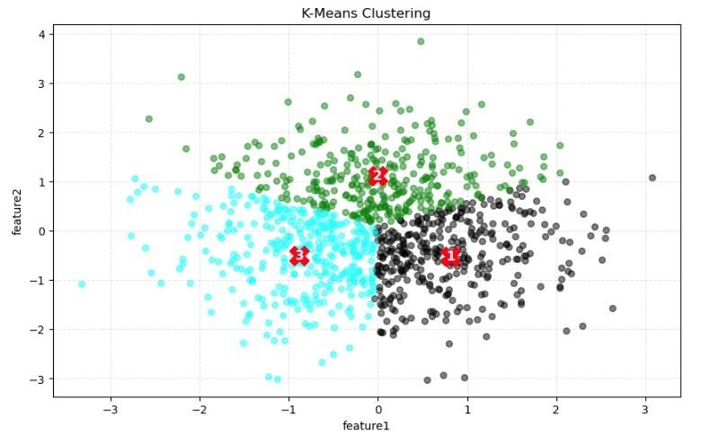
• Clusters: The data points are color-coded, likely to represent different clusters identified by the K-means algorithm. Typically, each color corresponds to one cluster. In this case, we have three distinct groups of data points represented by different colors (light blue, dark grey, and green).
• Centroids: The red numbers (1, 2, and 3) indicate the centroids of each cluster. These are the calculated mean positions of all the data points within a single cluster and are often considered the center of their respective clusters. The positioning of these centroids is crucial as the K-means algorithm assigns data points to clusters based on the shortest distance to these centroids.
• Data Distribution: The spread of the data points suggests the natural groupings within the dataset. From the plot, it seems that the light blue and green points are more mixed together, indicating that the separation between these two clusters might not be very clear. The dark grey points are more densely packed and appear to be well-separated from the other two clusters.
• Feature Axes: The feature1 axis (horizontal) and feature2 axis (vertical) are the two features based on which the clustering is done. These could be any quantitative aspects of the data, such as height, weight, income, etc., depending on the dataset being analyzed.
• Cluster Overlap: There appears to be some overlap between the clusters, especially between the clusters represented by the light blue and green points. This could suggest that the chosen features might not be entirely effective at separating the clusters distinctly, or it could reflect a natural overlap in the properties of the data points.

5. Evaluation Method

The Elbow Method is a powerful technique that helps us determine the optimal number of clusters (k) for K-means clustering. It does this by analyzing the Sum of Squared Distances (SSE) between data points and their respective cluster centroids. As we evaluate different values of k, we look for the point where the SSE curve begins to level off, resembling an elbow. This elbow represents the point beyond which increasing the number of clusters does not significantly improve the fitting of our model to the data. To put this method into practice, let’s consider the geyser dataset. By examining the SSE for various k values, we aim to identify where the curve transitions to a flatter slope, indicating the most appropriate number of clusters for our analysis.

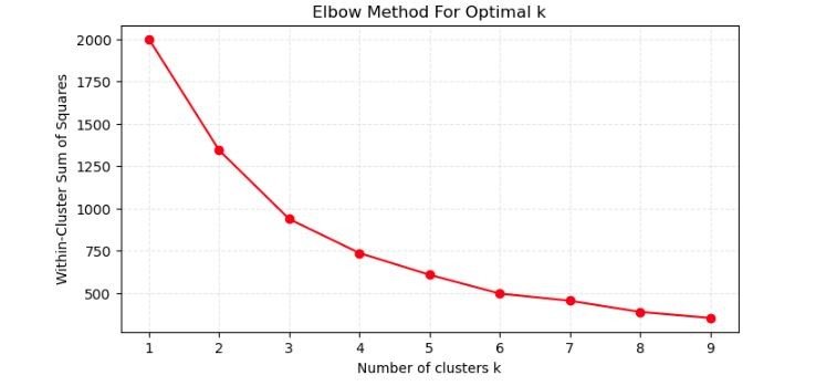
• X-axis (Number of clusters k): This represents the number of clusters used in the K-means algorithm. The graph shows values from 1 to 9 clusters.
• Y-axis (Within-cluster sum of squares): This axis shows the within-cluster sum of squares (WCSS), which is a measure of the compactness of the clusters. It is calculated as the sum of the squared distances between each data point and the centroid of its assigned cluster.
• Line: The line connects the WCSS for each number of clusters. As the number of clusters increases, the WCSS generally decreases because the clusters become smaller and tighter.
• Elbow Point: The elbow of the plot is the point where the WCSS begins to decrease at a slower rate as the number of clusters increases. This point is considered to be a good trade-off between the number of clusters and the cluster compactness.

Elbow seems to be around the point where k=3 or k=4. This suggests that increasing the number of clusters beyond 3 or 4 leads to diminishing returns in terms of decreasing the WCSS. Hence, the optimal number of clusters for this particular dataset might be 3 or 4 based on the Elbow.

Another Example

K-Means Clustering Visualization

The scatter plot displaying the output of the K-means clustering on a dataset.

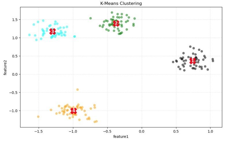
• Clusters: The different colors (light blue, green, grey, and orange) represent different clusters assigned by the K-means algorithm. The distribution of colors shows the grouping of the data points into four clusters.
• Centroids: The red numbers (1, 2, 3, and 4) mark the centroids of each cluster. These centroids are the mean position of all data points in the cluster and are used by the K-means algorithm to assign points to the nearest cluster.
• Feature Axes: The axes, feature1 and feature2, are the two features used for clustering. The clustering process places data points into clusters based on their similarity in this two-dimensional feature space.
• Cluster Characteristics: We observe that the clusters have varying density and separations. For example, the orange cluster appears more spread out, whereas the grey cluster is more compact. The centroids are located centrally within each of their respective clusters, which is characteristic of well-separated clusters.

Python Implementation for Another Example

The following code uses the `make_blobs` dataset from scikit-learn to generate a sample dataset and applies the K-means algorithm to cluster it.

from sklearn.datasets import make_blobs
#features and target
X, y = make_blobs(n_samples=200, centers=4, random_state=42)
#standard scale 
X = (X - X.mean())/X.std()

# K_Means for the clustering
km = K_Means(4)
# fitting model
km.fit(X)

# checking centroids
km.centroids

Elbow Method for Optimal k

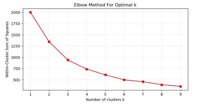
• Using the Elbow Method to identify the optimal number of clusters for K-means clustering.
• X-axis (Number of clusters k): Displays the number of clusters chosen for the K-means algorithm, ranging from 1 to 9.
• Y-axis (Within-cluster sum of squares): Indicates the within-cluster sum of squares (WCSS), which quantifies the compactness of the clusters. It is the sum of the squared distances between each data point and the centroid of the cluster it belongs to.
• Elbow Point: The graph is used to locate an “elbow” point where the rate of decrease in WCSS slows down significantly. In this plot, the elbow appears to be less pronounced, but there’s a subtle bend around k=4. This suggests that setting k=4 might be a reasonable choice for the number of clusters because beyond this point, the reduction in WCSS for each additional cluster is less significant.

6. Conclusion

K-means clustering is an important tool in machine learning for uncovering hidden patterns in data. It is particularly useful for exploratory data analysis, enabling the discovery of natural groupings within datasets. Through the iterative process of assigning data points to clusters and updating cluster centroids, K-means refines these groupings to optimize similarity within clusters and differences between them. The choice of the number of clusters, k, is pivotal, with methods like the Elbow and Silhouette providing guidance on the optimal cluster count.

Despite its simplicity, K-means faces challenges such as sensitivity to initial conditions and the potential for convergence to local optima. Nevertheless, when applied with considerations like data standardisation and careful initialisation, K-means clustering can yield insightful and actionable information across a multitude of applications.

Thank you for reading