The Perceptron: A Cornerstone of Neural Networks
The perceptron, introduced by Frank Rosenblatt in 1958, is one of the simplest yet most foundational models in machine learning. As a precursor to modern neural networks, it mimics the basic functionality of a biological neuron, serving as a linear classifier for binary classification tasks. This article explores the perceptron’s structure, its biological inspiration, its applications, and a practical implementation in Python for both classification and linear regression tasks.
1. Introduction to the Perceptron
In the realm of machine learning, the perceptron stands as a fundamental building block, paving the way for the complex neural networks that power today’s artificial intelligence. Designed to emulate the decision-making process of a biological neuron, the perceptron processes input data to make binary decisions, such as determining whether an email is spam or not. Its simplicity and interpretability make it an excellent starting point for understanding neural networks.
1.1 What is a Perceptron?
A perceptron is a single-layer neural network that takes multiple inputs, applies weights to them, adds a bias, and passes the result through an activation function to produce an output. Typically used for binary classification, it separates data into two classes using a linear decision boundary. While limited in its capacity to handle complex patterns, the perceptron is a critical stepping stone for understanding deep learning architectures.
1.2 Importance and Applications
The perceptron’s significance lies in its role as a foundational model in machine learning. It is widely used in educational settings to introduce neural network concepts and has practical applications in simple classification tasks, such as pattern recognition and basic image classification. Additionally, with modifications, the perceptron can be adapted for linear regression, showcasing its versatility.
2. Biological Inspiration
The perceptron draws inspiration from the human brain, specifically the behavior of neurons. By translating biological processes into a mathematical model, the perceptron captures the essence of how neurons process and transmit information.
2.1 Biological Neurons
In the human brain, neurons communicate through a network of synapses. A neuron receives signals via its dendrites, integrates them in the cell body, and, if the cumulative signal exceeds a threshold, sends an output signal through its axon to other neurons. This process, governed by synaptic plasticity and Hebb’s rule (“cells that fire together wire together”), forms the basis for learning and memory.
- Dendrites: Receive input signals from other neurons.
- Cell Body: Integrates incoming signals and determines whether to fire.
- Axon: Transmits the output signal to other neurons via synapses.
2.2 From Biology to Mathematics
The perceptron mirrors this biological process. Inputs (analogous to dendrites) are multiplied by weights (representing synaptic strength), summed with a bias, and passed through an activation function to produce an output. For classification, a step function typically determines whether the output is 0 or 1, while for regression, an identity function allows continuous outputs.
3. Structure of the Perceptron
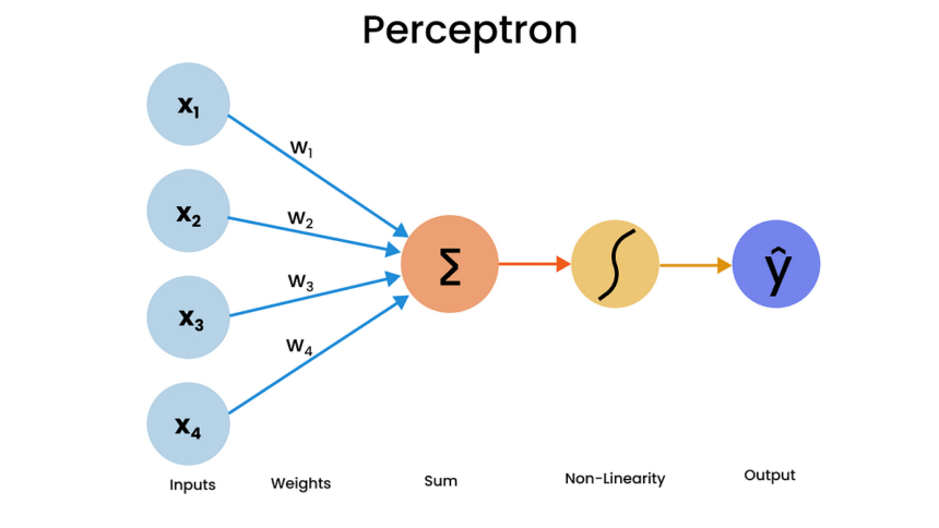
The perceptron’s architecture is straightforward, consisting of inputs, weights, a bias, a summation step, and an activation function.
3.1 Components of a Perceptron
- Inputs (x1, x2, …, xn): Represent features of the data, such as pixel values in an image.
- Weights (w1, w2, …, wn): Indicate the importance of each input, adjusted during training.
- Bias (b): Shifts the decision boundary, allowing flexibility in classification.
- Summation: Computes the weighted sum of inputs plus the bias: ∑(wi * xi) + b.
- Activation Function: Determines the output. For classification, a step function outputs 0 or 1; for regression, an identity function outputs the weighted sum directly.
3.2 How It Works
The perceptron calculates a weighted sum of its inputs, adds the bias, and applies the activation function. For binary classification, if the sum exceeds a threshold, the perceptron outputs one class (e.g., 1); otherwise, it outputs the other (e.g., 0). During training, weights and bias are updated to minimize errors, typically using a loss function like Mean Squared Error (MSE) for regression or misclassification error for classification.
4. Python Implementation
Below is a Python implementation of a perceptron adapted for both binary classification and linear regression, complete with data generation, training, and visualization.
4.1 Perceptron for Binary Classification
This implementation creates a perceptron for a binary classification task, using a step function as the activation function.
import numpy as np
import matplotlib.pyplot as plt

class PerceptronClassification:
    def __init__(self, learning_rate=0.01, n_iterations=100):
        self.learning_rate = learning_rate
        self.n_iterations = n_iterations
        self.weights = None
        self.bias = None
        self.losses = []

    def step_function(self, x):
        return np.where(x >= 0, 1, 0)

    def fit(self, X, y):
        n_samples, n_features = X.shape
        self.weights = np.zeros(n_features)
        self.bias = 0

        for _ in range(self.n_iterations):
            loss = 0
            for i in range(n_samples):
                linear_output = np.dot(X[i], self.weights) + self.bias
                prediction = self.step_function(linear_output)
                error = y[i] - prediction
                self.weights += self.learning_rate * error * X[i]
                self.bias += self.learning_rate * error
                loss += error ** 2
            self.losses.append(loss / n_samples)

    def predict(self, X):
        linear_output = np.dot(X, self.weights) + self.bias
        return self.step_function(linear_output)

# Generate synthetic classification data
np.random.seed(42)
X_class = np.random.randn(100, 2)
y_class = (X_class[:, 0] + X_class[:, 1] > 0).astype(int)

# Train the model
model_class = PerceptronClassification(learning_rate=0.01, n_iterations=100)
model_class.fit(X_class, y_class)

# Plot decision boundary
plt.scatter(X_class[:, 0], X_class[:, 1], c=y_class, cmap='bwr', alpha=0.5)
x1 = np.linspace(-2, 2, 100)
x2 = -(model_class.weights[0] * x1 + model_class.bias) / model_class.weights[1]
plt.plot(x1, x2, 'k-', label='Decision Boundary')
plt.xlabel('Feature 1')
plt.ylabel('Feature 2')
plt.title('Perceptron Classification')
plt.legend()
plt.grid(True, ls='--', alpha=0.2)
plt.show()
4.2 Perceptron for Linear Regression
This implementation adapts the perceptron for linear regression by using an identity activation function and minimizing Mean Squared Error (MSE).
import numpy as np
import matplotlib.pyplot as plt
import seaborn as sns
import scipy.stats as stats

class PerceptronLinearRegression:
    def __init__(self, learning_rate=0.01, n_iterations=100):
        self.learning_rate = learning_rate
        self.n_iterations = n_iterations
        self.weights = None
        self.bias = None
        self.losses = []

    def fit(self, X, y):
        n_samples, n_features = X.shape
        self.weights = np.zeros(n_features)
        self.bias = 0

        for _ in range(self.n_iterations):
            loss = 0
            for i in range(n_samples):
                prediction = np.dot(X[i], self.weights) + self.bias
                error = y[i] - prediction
                self.weights += self.learning_rate * error * X[i]
                self.bias += self.learning_rate * error
                loss += error ** 2
            self.losses.append(loss / n_samples)

    def predict(self, X):
        return np.dot(X, self.weights) + self.bias

    def mse(self, X, y):
        predictions = self.predict(X)
        return np.mean((predictions - y) ** 2)

    def r_squared(self, X, y):
        predictions = self.predict(X)
        mean_y = np.mean(y)
        ss_total = np.sum((y - mean_y) ** 2)
        ss_res = np.sum((y - predictions) ** 2)
        return 1 - (ss_res / ss_total)

# Generate regression data
def generate_regression_data(n_samples=200, n_features=1, noise=0.05):
    np.random.seed(42)
    X = np.random.rand(n_samples, n_features)
    true_weights = np.random.rand(n_features)
    y = np.dot(X, true_weights) + np.random.normal(scale=noise, size=n_samples)
    return X, y

X_reg, y_reg = generate_regression_data()

# Train the model
model_reg = PerceptronLinearRegression()
model_reg.fit(X_reg, y_reg)

# Plot loss during training
plt.plot(range(model_reg.n_iterations), model_reg.losses, color='black')
plt.xlabel('Iteration')
plt.ylabel('Loss')
plt.title('Loss During Training')
plt.grid(True, ls='--', alpha=0.2, color='black')
plt.show()

# Plot best fit line
y_pred = model_reg.predict(X_reg)
plt.scatter(X_reg, y_reg, color='black', label='Data points')
plt.plot(X_reg, y_pred, color='red', label='Fitted line')
plt.xlabel('X')
plt.ylabel('y')
plt.title('Perceptron Linear Regression')
plt.legend()
plt.grid(True, ls='--', alpha=0.2, color='black')
plt.show()

# Model evaluation
mse = model_reg.mse(X_reg, y_reg)
r_squared = model_reg.r_squared(X_reg, y_reg)
print(f"Mean Squared Error (MSE): {mse:.4f}")
print(f"R-squared: {r_squared:.4f}")

# Residual analysis
residuals = y_reg - y_pred
sns.residplot(x=y_pred, y=residuals, lowess=True, color="black")
plt.xlabel('Predicted values')
plt.ylabel('Residuals')
plt.title('Residual Analysis')
plt.grid(True, ls='--', alpha=0.3, color='black')
plt.show()

# Residual QQ plot and histogram
plt.figure(figsize=(10, 4))
plt.subplot(1, 2, 1)
qq = stats.probplot(residuals, dist="norm")
plt.scatter(qq[0][0], qq[0][1], color='black', alpha=0.5)
plt.plot(qq[0][0], qq[1][1] + qq[1][0]*qq[0][0], color='red', alpha=0.7)
plt.grid(True, ls='--', alpha=0.3, color='black')
plt.title('QQ Plot')

plt.subplot(1, 2, 2)
plt.hist(residuals, bins=30, color='black', edgecolor='black', alpha=0.7)
plt.xlabel('Residuals')
plt.ylabel('Frequency')
plt.title('Histogram of Residuals')
plt.grid(True, ls='--', alpha=0.3, color='black')
plt.tight_layout()
plt.show()

# Residual box plot
plt.figure(figsize=(3, 5))
sns.boxplot(y=residuals, color='black')
plt.title('Box Plot of Residuals')
plt.ylabel('Residuals')
plt.xlabel('Residuals')
plt.grid(True, which='both', linestyle='--', linewidth=0.5)
plt.show()
5. Evaluation and Analysis
The perceptron’s performance can be evaluated using metrics like accuracy for classification or MSE and R-squared for regression. Residual analysis further helps assess the model’s fit.
5.1 Classification Performance
For classification, the perceptron’s accuracy depends on the data’s linear separability. If the data is not linearly separable, the perceptron may fail to converge. Visualizing the decision boundary, as shown in the classification code, helps understand how well the model separates classes.
5.2 Regression Performance
For regression, the residual plots provide insights into model performance:
- Homoscedasticity: The residual plot shows constant variance, indicating a good fit.
- Normality: The QQ plot and histogram suggest that residuals are approximately normally distributed, with minor skewness at the tails.
- Outliers: The box plot identifies a few potential outliers, but their impact is minimal.
6. Advantages and Limitations
The perceptron offers several benefits but also has notable limitations.
6.1 Advantages
- Simplicity: Easy to implement and understand, ideal for beginners.
- Interpretability: Weights and bias provide clear insights into feature importance.
- Efficiency: Computationally lightweight, suitable for small datasets.
- Online Learning: Can update weights incrementally, ideal for streaming data.
6.2 Limitations
- Linear Limitation: Can only model linear relationships, failing on complex, nonlinear data.
- Convergence Issues: May not converge if data is not linearly separable.
- Limited Expressiveness: Lacks hidden layers, limiting its ability to capture complex patterns.
7. Conclusion
The perceptron, despite its simplicity, is a powerful tool for understanding the principles of neural networks. Its ability to perform binary classification and, with modifications, linear regression demonstrates its versatility. By drawing inspiration from biological neurons, the perceptron bridges biology and computation, offering a foundation for more complex models. While limited to linear problems, its ease of implementation and interpretability make it a valuable tool for learning and simple applications.
Thank you for reading!